Predictive CSI for 5G Link Adaptation

Closing the blind spot between channel reports. A 5G base station decides how fast to transmit to each user from the channel-quality (CQI) report the user sends back. Those reports arrive only periodically, and between them the scheduler holds the last value constant. In a moving network the channel has usually changed, so the transmission is matched to a channel that no longer exists. This feature predicts the next report, per user, and feeds that forecast into the scheduler's rate decision.

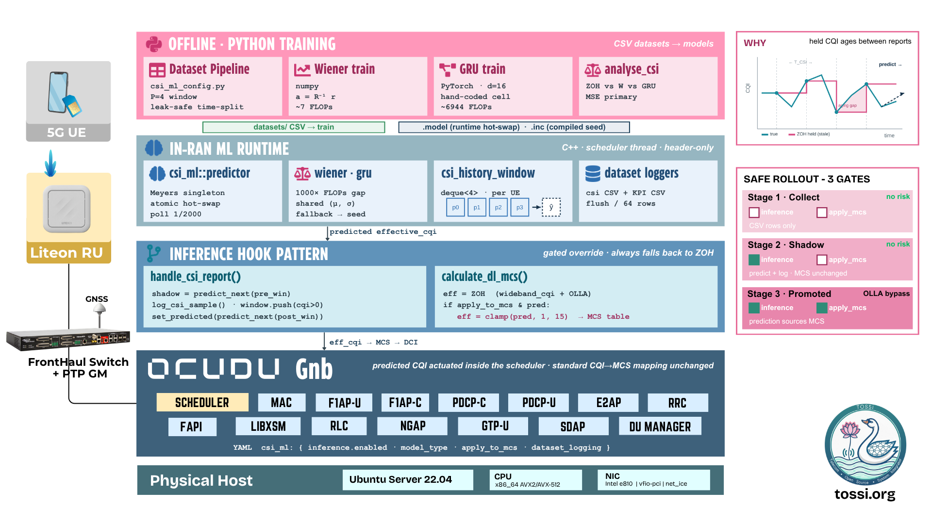
Architecture of the predictive CSI feature for OCUDU RAN. Offline Python training builds the models: a dataset pipeline (csi_ml_config.py, P=4 window, leak-safe time split), a Wiener trainer (numpy), a GRU trainer (PyTorch, d=16), and analyse_csi comparing ZOH, Wiener, and GRU by MSE. Each produces a runtime .model for hot-swapping and a compiled-in .inc seed. The in-RAN ML runtime (C++, on the scheduler thread) holds the csi_ml predictor, the Wiener and GRU cells, a per-UE csi_history_window (deque of 4), and dataset loggers. An inference hook pattern computes a predicted effective CQI in handle_csi_report and, in calculate_dl_mcs, either uses the ZOH baseline (wideband_cqi plus OLLA) or, when actuation is on, clamps the prediction into the MCS table; it always falls back to ZOH. The predicted CQI is actuated inside the OCUDU gNB scheduler with the standard CQI to MCS mapping unchanged. Side panels show why held CQI ages between reports, and the three-gate safe rollout (collect, shadow, promoted). — The predictive CSI architecture: offline Python training produces Wiener and GRU models, the in-RAN C++ runtime predicts a per-UE effective CQI on the scheduler thread, and a gated inference hook feeds it into rate selection, always falling back to the hold-last-report (ZOH) baseline.

Architecture in brief

The predictor sits alongside the scheduler's existing link-adaptation logic and is driven entirely by data the base station already has. There is no new interface to the user, no additional signalling, and no change to the radio standard, only the channel-quality value fed into rate selection changes.

Per-user prediction. Each connected user keeps a short rolling window of its most recent channel reports. When a new report arrives, the model forecasts the user's next value from that window. The forecast is cached and used for the following scheduling decisions, until the next real report refreshes it.

Two prediction engines, one interface. The same forecast can be produced by a lightweight linear predictor or by a compact neural predictor. Both plug into the same interface and are selected by configuration, so a deployment can choose the trade-off that suits its conditions.

Two CSI-prediction models operating through a common interface. Both the Wiener linear predictor and the GRU neural predictor consume the same four-report CQI input window and produce the same prediction output, while offering different compute and training characteristics. — Two prediction engines behind one interface. The Wiener linear predictor and the GRU neural predictor share the same four-report CQI input window and the same prediction output, and are selected by configuration, so a deployment picks the compute-versus-accuracy trade-off that suits its conditions.

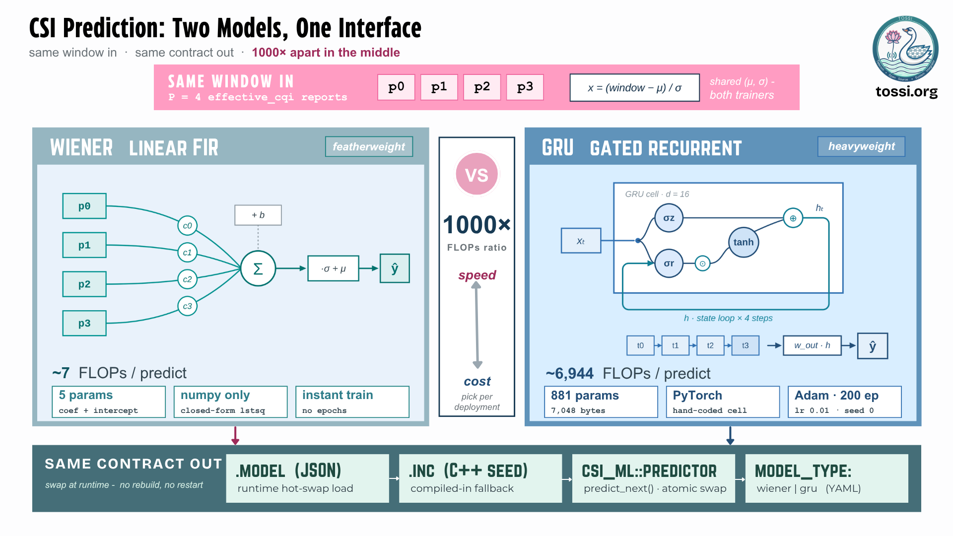
Runs inside the base station. Both models are compiled directly into the DU and execute as plain arithmetic, there is no external machine-learning runtime, no inference server, and no added latency on the scheduling path. Models can also be updated live, without restarting the base station.

Safe by construction. Whenever there is no confident forecast, early after a user connects, or when the input history is incomplete, the scheduler falls straight back to today's behaviour. The feature can never do worse than the current baseline.

Designed for mobility. The value of prediction grows precisely with how fast the channel changes. For a stationary user the last report is already a good estimate and there is little to gain. For a moving user, or when reports are spaced further apart, the last report goes stale quickly, and that is exactly the blind spot this feature fills.

What this brings

Better link adaptation. The scheduler transmits based on where the channel is heading, not where it last was, so the modulation and coding it chooses fits the real channel more often.
More efficient use of the same spectrum. Fewer over-optimistic transmissions that fail, and fewer over-cautious ones that leave capacity on the table, without any change to bandwidth, power, or hardware.
Strongest where it is needed most. The benefit scales with mobility and with the spacing of channel reports, targeting exactly the conditions where the conventional approach struggles.
Per-user, at cell scale. Every connected user gets its own forecast, so the improvement applies across a realistic multi-user cell rather than a single ideal link.
Zero deployment risk to adopt. It ships disabled, rolls out in reviewable stages, and always falls back to the current behaviour, so it can be evaluated safely before it ever influences a live transmission.
No standards impact. Fully within 3GPP: no new procedure, no message to the user device, no reconfiguration. It is an internal scheduler improvement.

Deployment and running guide

The feature rolls out in stages. Each stage is enabled independently in the DU configuration, so it can be validated before the next is turned on.

Clone the OCUDU-RAN repository and check out the dev branch, then build it (the predictor is compiled directly into the DU):

git clone https://github.com/TOSSI-Foundation/OCUDU-RAN
cd OCUDU-RAN
git checkout dev
./build.sh

Stage 1, Collect channel data

Enable dataset logging while inference stays off. Every channel report is recorded as one row, the recent history and the value that followed, building the examples the predictor learns from.

csi_ml:
  inference:
    enabled: false
  dataset_logging:
    enabled: true
    output_dir: ml/datasets
    scenario: collect_run

Run the base station with real users and move them through the conditions you want to cover (stationary, walking, driving), tagging each run with a distinct scenario. Each run produces a dataset file under output_dir.

Stage 2, Train the predictors

Train both models offline from the captured data. The linear model needs only numpy; the neural model additionally needs PyTorch.

# Linear predictor
python3 ml/training/train_export_csi_wiener.py ml/datasets/*.csv \
    --model-out ml/models/csi_wiener_seed.model \
    --inc-out   lib/scheduler/support/csi_ml_wiener_model.inc

# Neural predictor
python3 ml/training/train_export_csi_gru.py ml/datasets/*.csv \
    --model-out ml/models/csi_gru_seed.model \
    --inc-out   lib/scheduler/support/csi_ml_gru_model.inc

Each command produces a runtime model file (for live loading) and a compiled-in seed (baked into the binary on the next build). Both print a held-out comparison against the baseline so you can confirm the model is sound before deploying it.

Stage 3, Run in shadow mode

Turn inference on but keep actuation off. The base station now computes and logs a prediction for every report without changing any scheduling decision, zero risk, and it lets you confirm the live predictions match the offline evaluation.

csi_ml:
  inference:
    enabled: true
    model_type: gru          # 'gru' or 'wiener'
    gru_model_path: ml/models/csi_gru_seed.model
    apply_to_mcs: false      # shadow: logged, not applied
  dataset_logging:
    enabled: true
    output_dir: ml/datasets
    scenario: shadow_run

Stage 4, Promote to live

Once shadow results look right, enable actuation. The scheduler now sources channel quality from the prediction, still falling back to the baseline whenever no confident forecast is available.

csi_ml:
  inference:
    enabled: true
    model_type: gru
    gru_model_path: ml/models/csi_gru_seed.model
    apply_to_mcs: true       # live: prediction drives rate selection

Running the stack

Launch the core and base station together:

./run_stack.sh configs/csi_ml_example.yaml

On startup the active CSI-ML settings are printed, so every run is self-documenting, you can see at a glance which model is live and whether it is shadowing or actuating.

Updating a model without downtime

Point the model path at a new file and replace it in place; the base station detects the change and swaps the model atomically, with no restart and no interruption to service.

Results

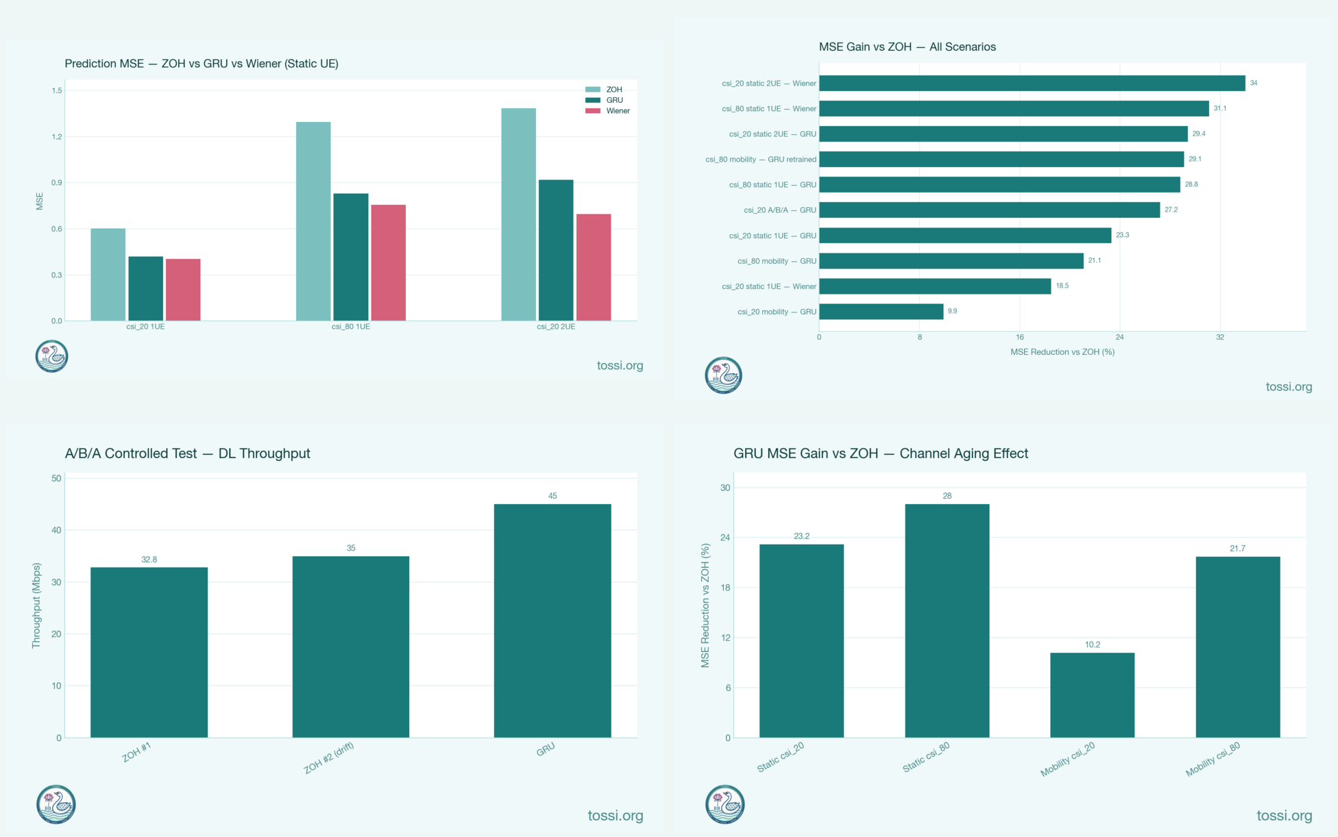
Benchmarking was performed on mobile user equipment in a controlled environment, comparing the predictive scheduler against the conventional hold-last-report baseline under matched conditions. To separate a genuine improvement from run-to-run variation, the baseline was measured repeatedly to establish a noise floor, and the predictive configuration was evaluated against it on identical traffic and radio conditions.

The evaluation looks at two layers:

Prediction quality, how closely the forecast tracks the channel quality the user actually reports next, compared with holding the last report.
Delivered performance, the downlink throughput and error rate the user experiences with the predictor driving rate selection, against the same baseline.

Four benchmark charts for predictive CSI. Top left, prediction MSE for zero-order hold (ZOH, hold last report) versus the GRU and Wiener predictors on static UE across csi_20 and csi_80 report spacings and one and two UEs, where both predictors have lower MSE than ZOH. Top right, MSE reduction versus ZOH ranked across all scenarios, from 9.9 percent to 34 percent. Bottom left, the A/B/A controlled downlink throughput test: ZOH at 32.8 and 35 Mbps versus GRU at 45 Mbps. Bottom right, GRU MSE reduction versus ZOH by channel-aging condition (static and mobility, csi_20 and csi_80), showing the gain grows with report spacing. — Predictive CSI benchmarks against the hold-last-report baseline (ZOH). The GRU and Wiener predictors lower prediction MSE across scenarios (9.9 to 34 percent), and the A/B/A controlled test shows the GRU lifting downlink throughput from roughly 33 to 45 Mbps, with the largest gains where reports are spaced further apart.

Notes

The feature is disabled by default and has no effect until explicitly enabled.
It changes only the channel-quality value fed into the existing, standard rate-selection logic; the modulation and coding tables, the radio interface, and all signalling are untouched.
Prediction helps in proportion to how fast the channel changes. In near-static conditions the baseline is already close to optimal, and the feature is designed to match it there, not regress it.